CFD Modeling of a Mixing Tee – Part 2: Predictions of Temperature Fluctuations
by Dave Dewees, Zumao Chen and L. Magnus Gustafsson
This is the second part of a 2-part blog. In Part 1, the stress-blended eddy simulation (SBES) and large eddy simulation (LES) approaches for simulating turbulence have been validated against test data obtained from a mixing tee. In this part, the SBES approach is used to predict temperature fluctuations in a mixing tee where light gas oil mixes with a recycled gas. Depending on the characteristics of the streams being mixed (momentum and temperature), protection from rapid temperature variations occurring even at steady-state bulk flow conditions is a necessity. While a CFD model can predict these temperature variations with good fidelity as shown in Part 1 of this blog, once a problem is found, the same CFD model can also be used to design solutions that protect the piping at the mix point. Here thermal sleeve length is optimized through use of the validated SBES technique described in Part 1.
Mixing tees are widely used in the petrochemical industry, in which two fluid streams with different physical and/or chemical properties mix together. When there is a large temperature difference between the two streams, large metal temperature fluctuations can occur in the region where the two streams meet if proper design steps are not taken. The temperature fluctuations in the metal may lead to thermal fatigue of the pressure boundary piping. If through-wall cracking occurs, the fluid may leak, possibly causing a fire and damage. It is therefore imperative to make sure that the temperature fluctuations are such that the piping system can withstand them. Options can include improving the mixing of the two streams to reduce the temperature fluctuations through redesign of the piping system such that the momentum ratio of the two fluid streams is favorable to rapid mixing, or to install devices that protect the pressure boundary piping, e.g., injection quills or thermal sleeves in the region where the temperature fluctuations are higher than a thermal fatigue threshold. This region includes the T-junction and a length of several to many main pipe diameters downstream from the T-junction. For sleeves, there are different approaches to determine the needed sleeve length downstream from the T-junction, which are briefly discussed here.
Empirical correlations in the literature may be used to estimate mixing effectiveness or the uniformity of the fluid concentrations over the pipe cross section downstream from the T-junction [1], whereby the length of the pipe that needs protection can be determined. However, these correlations were developed based on experiments typically using air or water as working fluids and a chemical agent as the tracer to indicate the mixing uniformity. The temperature differences between the two fluid streams in these experiments were usually small. Therefore, these correlations should be used with caution when the actual fluid conditions are well outside of the range in which the correlations were developed.
Computational fluid dynamics (CFD) modeling, such as wall-resolved large eddy simulation (LES), can provide accurate predictions of the mixing behavior, including velocity, concentration and temperature fields, in a mixing tee [2, 3]. The variations of the transient fluid temperature can therefore be used to identify a location in the main pipeline, after which the maximum temperature difference is less than a given value.
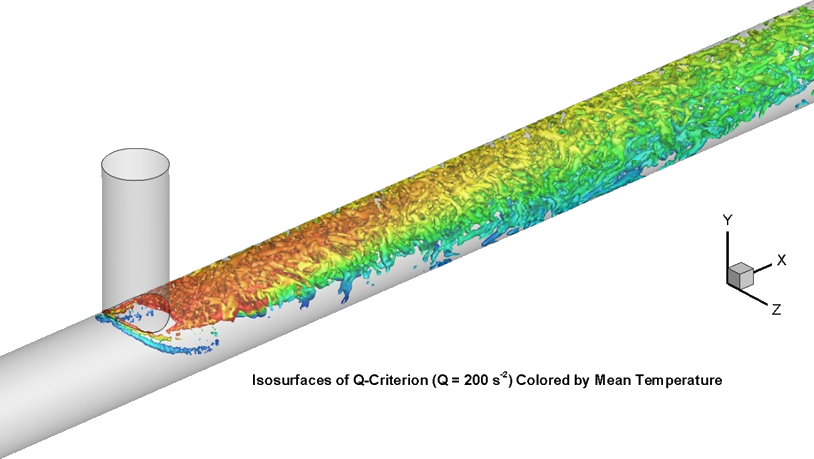
In the following, a mixing tee that blends light gas oil with a recycled gas is modeled using SBES. The light gas oil temperature is 600°F and the recycled gas temperature is 960°F. The operating pressure of the mixing tee is 1,700 psig. The large temperature difference between the two streams is expected to cause large temperature differentials downstream of the junction, which may lead to thermal fatigue of the pipeline if the pipe is not properly protected.
Figure 1 shows the distributions of the instantaneous temperature and root-mean-square-error (RMSE) temperature on a vertical plane through the pipe centerline. The instantaneous temperature distribution shows intensive mixing between the two streams downstream of the junction. The momentum of the branch flow is much lower than that from the main pipe inlet: the latter sweeps past the former and forces the branch flow to bend towards the top portion of the horizontal pipe. The RMSE temperature distribution indicates large temperature fluctuations at the interface where the two streams come into contact. Downstream of the junction, the fluctuations are relatively small in the bottom portion of the pipe and the recycled gas tends to stay in the upper section.
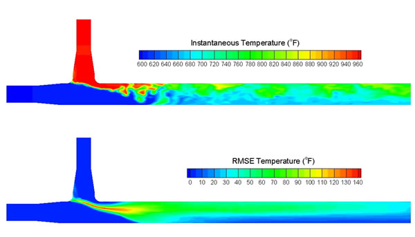
Figure 1: Temperature Distributions on a Vertical Plane through Pipe Centerline
Figure 2 shows the instantaneous temperatures at different locations. Temperatures at four locations are presented. Looking in the main flow direction, the locations at the 12, 3, 6 and 9 o’clock positions are denoted as “top”, “right”, “bottom” and “left”, respectively, in the figure. Distance, x, is the distance from the junction and D is the main pipe diameter.
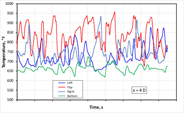
Figure 2: Instantaneous Temperature as a Function of Flow Time: x = 4 D
The temperature sampling locations are 1 mm away from the inner surface of the pipe. The results show that the minimum temperature is always at the bottom of the pipe and the maximum temperature is usually at the top of the pipe. The maximum temperature difference for the pipe cross section at x = 4 D is 340°F.
Figure 3 shows the maximum temperature differences at different locations downstream of the junction. As the distance from the junction increases, the maximum temperature difference decreases. At x = 6 D, the maximum difference is 253°F, while at x = 10 D, the maximum difference is 209°F.
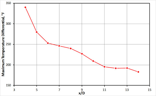
Figure 3: Maximum Temperature Difference along Main Pipeline
While the actual temperature of the exposed metal will depend on the frequency of the temperature fluctuations, the results shown in Figure 3 illustrate how CFD modeling results can be used to determine the distance from the junction, over which the temperature fluctuations are higher than the thermal fatigue threshold and the pipe section needs a thermal sleeve. For best results, the pipe metal is included in the CFD model directly (although not shown here). The modeling results also show a stratified flow of the two fluid streams downstream of the junction, where the recycled gas tends to stay at the top part of the pipe and the light gas oil tends to remain at the bottom part, even after ten pipe diameters. However, the maximum temperature difference is only 209°F at x = 10 D.
References
[1] Forney L.J., Jet injection for optimum pipeline mixing, Encyclopedia of Fluid Mechanics, Vol. 2, Chapter 25, 660-690, 1986.
[2] Becht Internal Document, CFD modeling of a mixing tee, 2018.
[3] Smith B.L., Mahaffy J.H. and Angele K., A CFD benchmarking exercise based on flow mixing in a T-junction, Nuclear Engineering and Design, 264, 80-88, 2013.
If you have a question relating to this blog, you may post a comment for the author at the bottom of this page. If you would like to submit an Information Request please click below: