How Machine Learning Expands the Value of Smart Instrumentation in Refineries

By Orion Burl and Frank Sapienza
Machine learning helps refineries determine which process conditions most strongly affect corrosion by analyzing continuous sensor data alongside operating variables. This enables better-informed integrity decisions than traditional inspection-only approaches.
Key takeaways
- Continuous UT sensors provide higher-frequency corrosion data than manual inspections.
- Machine learning identifies which process variables most influence corrosion rates.
- Gradient Boosted Decision Trees model nonlinear refinery data effectively.
- SHAP analysis improves interpretability of corrosion models.
- Model accuracy improves as historical sensor data increases.
Applying machine learning to real refinery problems
As refineries gain access to increasingly large volumes of data, opportunities are growing to use modern machine learning techniques to draw meaningful conclusions. While Large Language Models tend to capture mainstream attention, the fundamental learning algorithms behind them can be just as powerful when applied to real refinery challenges.
One area where these techniques are particularly valuable is mechanical integrity management. Understanding the correlation between process variables and corrosion is fundamental to managing mechanical integrity, but many plants still rely solely on traditional (manual) ultrasonic thickness (UT) inspection programs based on infrequent and inconsistent measurements. When contrasted to employing an installed UT sensor continuous monitoring strategy, owner-users see significantly improved measurement accuracy and frequency; however, determining which variables truly drive mechanical integrity risk remains a challenge. Machine learning helps close that gap.
To demonstrate this, we used a Gradient Boosted Decision Tree model to effectively identify which process variables most significantly impact the corrosion rate in a depropanizer. Below, we break down how the model was built – starting with data preparation and feature engineering, moving through training and testing, and ending with how we drew results from the trained model.
Preparing refinery data for machine learning modeling
The key to any good model is validated input data. Anyone familiar with refinery thickness data or process instrumentation measurements will understand the need to review this data for outliers, instrument errors, and other artifacts than could affect the end result.
Corrosion rate
We worked with Sensor Networks, who installed three fully wireless, single-point microPIMS (Permanently Installed Monitoring Systems) sensors to obtain thickness values in the depropanizer. An example of an installed microPIMS is shown in Figure 1. Plants often have more than 100 sensors installed across different units, representing a high volume of data. These sensors have a built-in temperature element that measures the skin temperature used to calculate temperature-adjusted thickness; however, these particular locations were not insulated, which caused swings in surface temperature measurements. Additionally, there were step changes in sensor thickness due to turnaround and sensor maintenance activities. By accounting for these issues, we were able to move from the initial inconsistent thicknesses (Figure 2, left) to improved temperature-adjusted thicknesses (Figure 2, right). This allowed us to calculate a corrosion rate that could serve as our model’s predicted value (Figure 3).

Figure 1: Example of a microPIMS sensor installed on a vessel
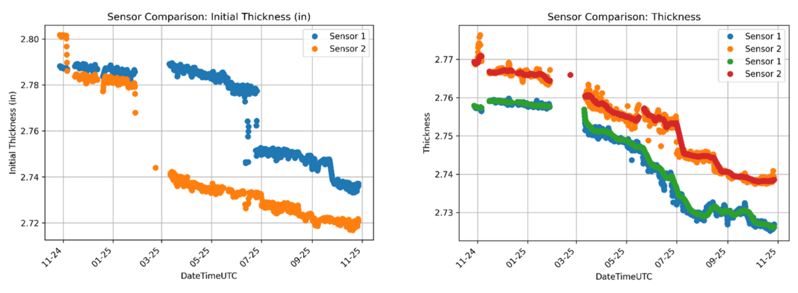
Figure 2: Comparison of initial sensor thickness (left) vs. temperature-adjusted thickness (right)
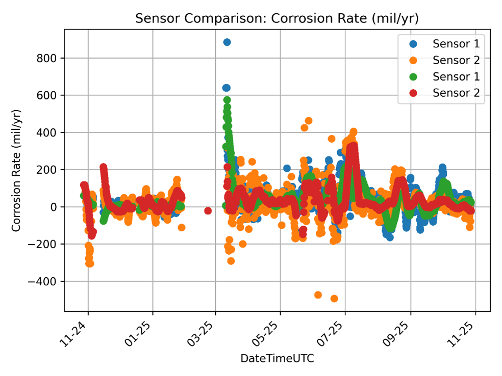
Figure 3: Corrosion rate trends of sensors over time
Process values
Process variables for study were chosen based on integrity operating window (IOW) variables in collaboration between the process engineer and corrosion engineer. IOWs are limits set on process variables to control corrosion; therefore, these parameters are most likely to correlate with measured corrosion rates. The first step in cleaning the process data was to remove invalid values and periods of abnormal unit operation, as defined by site engineers. Due to the difference in available data frequency between the corrosion rate and process variables, there was a large temporal resolution mismatch. We accounted for this by averaging and interpolating to obtain values at the same time stamps as corrosion rates. This allowed us to create usable input/output pairs for modeling.
It is important to note that there will always be some limitation in drawing a direct relationship between a process variable change and a corrosion rate response. Because corrosion rate responds slowly, this method is best suited to evaluating the impact of variables that shift over longer periods, not brief excursions. Additionally, lab values in process historian (PI) will persist until a new value is taken, which can obscure the true real-time value. Finally, the nonlinear nature of the model is meant to allow for understanding of the interacting effects of different process variables. Each process variable was also evaluated visually, as seen below in Figure 4, to provide a qualitative method confirming the existence of any relationships.
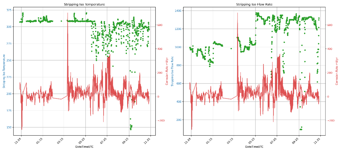
Figure 4: Qualitative view of selected process variables (stripping ISO temperature and flow rate) vs. corrosion rate
Developing a machine learning model to predict corrosion behavior
Algorithm decision
In general, a supervised regression machine learning algorithm takes a target output, y (in this case, corrosion rate), and a set of inputs, x₁…xₙ (process values such as temperature, acid strength, etc.), and develops a model for the relationship between them such that y = f(x₁…xₙ). Machine learning algorithms excel at representing extremely complex, nonlinear models, accounting for input relationships that would be too complicated for a traditional algebraic model. The algorithm takes in known data to train itself, determining parameter weights that are used in a final prediction. After training is complete, any set of values for the input parameters can be used, and a prediction for the output value can be made.
For this application, we selected a Gradient Boosted Decision Tree because it:
- Accurately models complex, non-linear processes
- Performs better with limited data and is less prone to overfitting compared to other algorithms
- Offers input transparency, allowing for better calculation of relevant feature importance
Testing and training
We employed two training methods:
- Typical split: Dividing the data into training and testing sets to evaluate model generalization
- Full regression: Using all available data to maximize the training volume
A grid search was conducted across multiple rolling average durations. For each set of training inputs, we performed a k-fold cross-validation with grid search on Boosted Tree hyperparameters, varying the depth and number of trees in the model. Training on multiple subsets of data helped ensure a robust model. In addition to the traditional training/test analysis, we also ran a pure regression analysis without a test data split. While it increases the likelihood of overfitting and reduces predictive reliability, this approach is more useful for our interpretive goals because it allows us to evaluate variable influence and determine relative feature importance.
We also experimented with the number of inputs analyzed, starting with a full set of 22 variables. From there, we tested models with different subsets based on the type of input. Several variables had only a minimal effect on the output; however, removing them still reduced overall model performance. Although the relative ranking of feature importance stayed consistent across subsets, the total model error increased when inputs were removed. This suggests that some variables interacted with others in ways that contributed meaningfully to the model, even if their standalone impact was small.
In addition, reducing the number of inputs also decreased the number of distinct data points available to differentiate operating states. Due to the general variance of the system, a similar set of values could correspond to very different corrosion rates, which ultimately diluted the influence of those inputs.
Evaluating model results using SHAP and feature importance
To understand which process variables most strongly influence corrosion rate, we used a Shapley Additive exPlanations (SHAP) plot. An individual SHAP value illustrates how much a given feature contributes to the model’s predicted corrosion rate by approximating predictions across many combinations of input values and measuring the change associated with that feature. We repeated this calculation for every feature and input point, summarized in Figure 4 (left) below. For each point, the color represents the value of the feature, while the distance from the center is the magnitude and direction of its impact.
To compare features more directly, we assumed a generally monotonic relationship between each feature and its impact on corrosion rate. This allowed us to use the Spearman correlation coefficient between the feature and its impact. For the most significant features, importance remained consistent even as more data was added. Figure 4 (right) shows the Spearman correlation for each feature, where the magnitude reflects how consistently the directionality holds. For the highest positive correlations, we can confidently expect that as the process value increases, the corrosion rate will also increase. Because the Spearman correlation relies on relative rank, it is less susceptible to outliers – an advantage given the variability in thickness data.
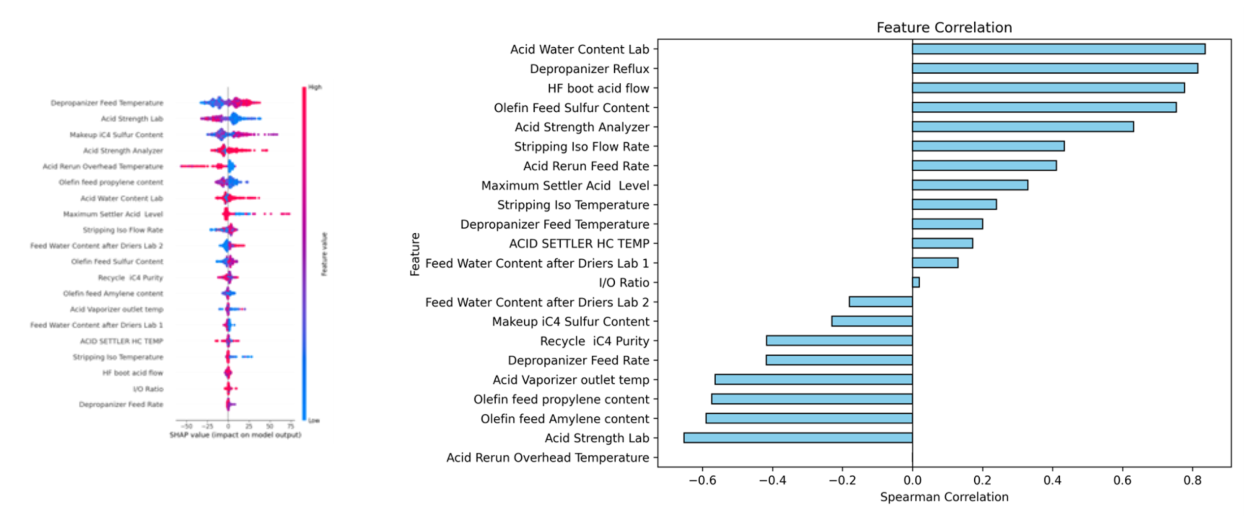
Figure 5: SHAP plot (left) and Ranked Importance chart (right) help identify the most important process variables
What machine learning reveals
Based on our analysis, we can identify which process conditions have the most meaningful impact on corrosion rate, compare these with expectations rooted in corrosion knowledge, and provide evidence to support potential operational adjustments. However, limitations in the underlying thickness data coupled with general instrumentation issues and the infrequency of lab measurements mean that exact corrosion rate predictions should be interpreted with caution, and some influential factors may not be fully captured. The smart sensors were installed in October of 2024, so one year of data was used for analysis. As more data becomes available, the model can be retrained and continue to improve, providing more reliable results.
Machine learning techniques like this can be applied to many refinery challenges, from corrosion modeling to process optimization – especially when extensive, high-quality data is available to allow for ample training opportunities. Integrating existing process knowledge or other domain experience with data-backed insights helps reinforce hypotheses or identify new ideas to consider. Prediction models can also be developed and updated in real time as new data comes in, integrating with any step in the operations or data engineering process.
Similar models can be applied across multiple refineries to highlight common patterns and potential shared solutions. Ultimately, any process where an output variable is influenced by a set of input parameters and supported by a large dataset can benefit from machine learning to better anticipate and optimize performance.
Interested in applying machine learning techniques at your site?
The methods highlighted in this blog – including data preparation, feature engineering, supervised modeling, and model interpretation – are core components of Becht’s new AI and ML Fundamentals for Refinery Engineers course. This course focuses on practical refinery use cases (including corrosion modeling) and is designed to help engineers confidently apply machine learning to real operational challenges. Contact Becht to register or discuss how these approaches could be applied at your facility.
Like what you just read? Join our email list for more expert insights and industry updates.